Use of Basic Elements III – Orthogonal Collocation on Finite Elements

On this page

This example shows how to implement orthogonal collocation by hand in MOSAICmodeling.

Model description

The model is fairly simple as it consists of only one differential equation:

$\frac{\mathrm{d}z}{\mathrm{d}t} = z^2 - b \cdot z + 1.$

Therein, $z$ is the differentiated variable, $b$ is a parameter, and $t$ is time. If we apply orthogonal collocation on this differential equation, we obtain

$\sum_{j=0}^{NJ}a_{j,c}\cdot z_{c=j} = z_{c}^2 - b \cdot z_c + 1.$

Finally, if we divide the time horizon into several finite elements, we have the following discretization. In addition, we need a equation that enforces continuity between the finite elements:

$\sum_{j=0}^{NJ}{a_{j,c}\cdot z_{c=j,i}}= ((z_{c,i})^{2} - b \cdot z_{c,i} + 1)\cdot h_{i}, \\[2ex] z_{c=3,i}=z_{c=0,i+1}.$

In the discretized equations, $a_{j,c}$ is a collocation coefficient equal to the derivative of the j-th lagrange basis polynomial at the c-th collocation point. The index $i$ marks the finite elements and $h_i$ is the length of the i-th finite element. Optionally, the time can also be discretized although it usually does not explicitly appear in chemical engineering applications:

$t_{i,c}=t_{i-1,c=NC}+\tau_{c} \cdot h_{i}.$

Model workflow

Notation

Once again, we begin by setting up the notation. Therefore, perform the following steps:

Go to the Notation tab in the “Model” section
Add a description of your notation
Add the base names below by clicking on “+ Name” at the bottom, entering these names, adding a description of the variable and confirming it
Go to the Indicies tab and add the index below
Once you have added all variables and symbols, click on “Save” at the top of the editor and save your notation at a suitable location in your folder structure

Base names

$\tau$ , collocation point
$a$ , collocation coefficient, i.e., derivative of lagrange basis polynomial
$b$ , parameter
$h$ , length of finite element
$t$ , time
$z$ , state variable

Indices

$c$ , Index of collocation points 1..NC
$i$ , Index of finite elements 1..NI
$j$ , Index of lagrange basis polynomials 1..NJ

The notation is available with ID 8480.

Equations

Go to the Equation tab. Proceed as follows:

Load the notation you just created
Add an informative description of the current equation
Type the first model equation in LaTeX style into the window MosaicTex. For the differential operator, you must use \diff{Var}{IndependentVariable}
Save the equation at a suitable location in your folder structure
Click on “New” at the top of the editor and repeat the steps 1 and 2
Enter the remaining model equations for the discretized forms and save them as well

The equations have IDs 8481, 8486, 8490, 8497, and 8492.

Equation systems

Now, we will combine our equations to three equation system. To this end, go to the Equation System tab and carry on as described below:

Load your notation from above
Add a suitable description
Go to the tab Connected Elements and click on “+ EQU/EQS” at the bottom of the editor
In the opening popup window, select your differential equation and confirm
Save your equation system with this single differential equation
Repeat the steps 1-5 with the single discretized equation and the discretized form with finite elements in combination with the continuity equation

The resulting three equation systems have the IDs 8482, 8487, and 8491.

Simulation workflow

Start by going to the “Simulation” section of MOSAICmodeling.

Equation systems and Indexing

Here, we describe the following steps in a simultaneous way. In MOSAICmodeling, you would rather set up the simulations sequentially: go to the tab Equation System and select the first of your newly saved equation system from above. For this system, you do not have to specify and indices.

For the discretized version of the equation system, you need to specify the number of collocation points (NC = 3) and the number of lagrange basis polynomials (NJ = 3). For the discretized version on multiple finite elements, you also need to set an appropriate number of finite elements. Here, we choose NI = 5. For the latter two systems, click on Confirm Index Data to instantiate the systems.

Specifications and solution

Go to the tab Specifications and then select the tab Variables. For the ODE system, proceed as follows:

Add a helpful description of the simulation
In the specification window, you can see all possible variable classifications. Select ALL VARIABLES at the top. You should now see the four variables that are part of your model
Change the entry in the column Type for $b$ to Design Value
Change the type classification of the variables $z$ to state variable. The variable $t$ should already be classified as differential value. Your degree of freedom should now be zero
Assign the values given in Table 1 to the three variables
Save your variable specification by clicking on the “Save” button above the calculation of the degrees of freedom
Save your simulation by clicking on “Save” at the top of the editor

For the discretized ODE, do as follows:

Add a helpful description of the simulation
In the specification window, you can see all possible variable classifications. Select ALL VARIABLES at the top. You should now see the four variables that are part of your model
Change the entry in the column Type for $b$ , $a_{j=0,c=1}$ – $a_{j=3,c=3}$ , $b$ , $h_{i=1}$ , $t_{i=0,c=NC}$ , and $z_{c=0}$ to Design Value
Assign the other six variables $t_{i=1,c=1}$ – $t_{i=1,c=3}$ and $z_{c=1}$ – $z_{c=3}$ as ITERATION_VALUE
Assign the values given in Table 1 to the variables
Save your variable specification by clicking on the “Save” button above the calculation of the degrees of freedom
Save your simulation by clicking on “Save” at the top of the editor

For the discretized ODE on finite elements, take the following steps:

Add a helpful description of the simulation
In the specification window, you can see all possible variable classifications. Select ALL VARIABLES at the top. You should now see the four variables that are part of your model
In addition to the same $a_{j,c}$ , $b$ , and $t_{i=0,c=NC}$ from the previous simulation, change the entry in the column Type for $h_{i}$ and $z_{c=0,i=1}$ to Design Value
Assign the remaining $t_{i,c}$ and $z_{c,i}$ – $z_{c=3}$ as ITERATION_VALUE
Assign the values given in Table 1 to the variables
Save your variable specification by clicking on the “Save” button above the calculation of the degrees of freedom
Save your simulation by clicking on “Save” at the top of the editor

The simulations are available with IDs 8484, 8489, and 8494; the respective variable specifications have IDs 8483, 8488, and 8493. The solutions are compared in Figure 1. They were obtained by plotting the ODE solution against the solutions of the other two cases. Note that MOSAICmodeling does not automatically generate plot functions for discretized systems. These must be written by the user.

Table 1: Overview of design values and initial conditions.

Name	Description	Value / Initial guess	Solution
$b$	Parameter	2.0
$z$	State variable	-3.0
$\tau_{c=1}$	Collocation point 1	0.15505
$\tau_{c=2}$	Collocation point 2	0.6449
$\tau_{c=3}$	Collocation point 3	1.0
$a_{j=0,c=1}$	Derivative of lagrange basis polynomial	-4.1394
$a_{j=1,c=1}$	Derivative of lagrange basis polynomial	3.2247
$a_{j=2,c=1}$	Derivative of lagrange basis polynomial	1.1678
$a_{j=3,c=1}$	Derivative of lagrange basis polynomial	-0.2532
$a_{j=0,c=2}$	Derivative of lagrange basis polynomial	1.7394
$a_{j=1,c=2}$	Derivative of lagrange basis polynomial	-3.5678
$a_{j=2,c=2}$	Derivative of lagrange basis polynomial	0.7753
$a_{j=3,c=2}$	Derivative of lagrange basis polynomial	1.0532
$a_{j=0,c=3}$	Derivative of lagrange basis polynomial	-3.0
$a_{j=1,c=3}$	Derivative of lagrange basis polynomial	5.532
$a_{j=2,c=3}$	Derivative of lagrange basis polynomial	-7.532
$a_{j=3,c=3}$	Derivative of lagrange basis polynomial	5.0
$h_{i=1}$	Length of finite element (for case 2)	1.0
$t_{i=0,c=NC}$	Initial time (for case 2)	0.0
$z_{c=0}$	Initial condition of discretized state variable (for case 2)	-3.0
$t_{i,c}$	Times at other collocation points	0.5	0.15505, 0.6449, 1.0
$z_c$	Solution at other collocation points	0.0	-1.657, 0.032, 0.207
$h_{i}$	Length of finite element (for case 3)	0.2
$z_{c=0,c=NC}$	Initial time (for case 3)	0.0
$z_{c=0,i=1}$	Initial condition of discretized state variable (for case 3)	-3.0
$t_{i,c}$	Times at other collocation points	0.5	See results after code generation
$z_{c,i}$	Solution at other collocation points	-1.5	See results after code generation

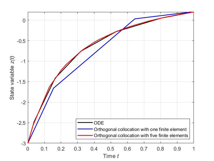
Figure 1: Comparison between the three different cases. The solution with one finite element is stable, but differs significantly from the ODE solution. With more finite elements, the solution is approximated much better.